

diffraction
electron transfer
electromagnetic field
energy level
energy level diagram
energy transfer and energy transfer with upconversion
excited state absorption
fluorescence
green fluorescent protein
Kerr effect
multi-photon absorption
nondegenerate two-photon absorption
nonlinear index of refraction
nonparaxial approximation
optically thick sample
paraxial approximation
phosphorescence
plane wave
photo-activated material
photodynamic therapy
pump probe experiment
quantum dots
relaxation
reversible saturable absorption
saturable absorption
self-quenching
single-photon absorption
slowly varying envelope approximation
split-step numerical method
STED microscopy
stimulated emission
three-photon absorption
two-photon absorption
upconversion
Z-scan

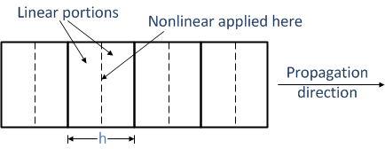
The split-step method is a numerical method that can be used, for example, for finding a numerical solution of scalar Maxwell’s propagation equations having both linear and nonlinear terms. Each numerical step in the propagation direction is composed of applying two half-step linear operators (linear portions) and one one-step non-linear operator in between the linear portions towards a solution at a previous numerical step.
In the scalar form of Maxwell’s equations, the electric field of a cylindrical beam of light propagating in the z-direction can be written as
| E(z,t) = φ(z,t) exp[ -iωt ] |
However, the phase of φ(x,y,z,t) varies rapidly along the propagation direction (usually specified as the z-direction). This rapid phase variation is not important for many types of problems and can be removed by introducing a slowly varying field A(z,t) and constant k, such that
| φ(z,t) = A(z,t) exp[ ikz ] |
It is assumed that A(z,t) varies slowly in the propagation direction z as well as the other two directions and time t,
| | ∂A/∂z | << k | A | | ∂A/∂t | << ω | A | |
which implies, for example, that
| ∂2A/∂z2 ≈ 0 |
This reduces a second order differential equation to a first order equation that is easier to solve.
| ∂A(z,r,t) /∂z = (L + N) A(z,r,t) |
where L is comprised of linear terms (e.g., background absorption, diffraction and dispersion) and N is comprised of nonlinear terms (e.g., Kerr term, single- or multi-photon absorption). Applying both operators at once is not possible during numerical integration. An obvious shortcut will be to apply the operators in turn as follows
| A(z + h,r)= exp[L h] exp[N h] A(z,r) |
However, this may drastically decrease accuracy of the numerical solution as the linear and nonlinear operators do not commute:
| exp[L + N] ≠ exp[L] exp[N] |
To achieve a better accuracy one can make splitting mode efficient (a variation of standard Strang splitting, second order accuracy):
| exp[L + N] ≈ exp[L/2] exp[N] exp[L/2] |
Assume the propagation direction is divided into increments of length h as shown below.
For a propagation step of length h the solution of the differential equation at A(z + h) is
| A(z + h, r) ≈ exp[L h/2] exp[∫ N(z’) dz’] exp[L h/2] · A(z,r) |
The nonlinear portion for the entire increment h (the middle integral factor shown above) is applied at the center of the increment and between the two linear portions. The integral of N(z’) is calculated over the whole increment h from z’ = z to z’ = z + h.
Several variations of this method exist. Depending on the problem at hand (e.g., complexity of nonlinear or linear operators), one can surround the linear step with two nonlinear half-steps:
| A(z + h, r) ≈ exp[N h/2] exp[∫ L(z’) dz’] exp[N h/2] · A(z,r) |
A higher (fourth) order can be also applied as follows
| A(z + h, r) ≈ SS2(ah) • SS2({1-2a}h) • SS2(ah) • A(z,r) |
where SS2 (h) = exp(N h / 2) • exp ( ∫ L(z’) dz’) • exp (N h / 2) is a split-step operator of the second order and a=(2+21/3+2-1/3)/3 is a constant.
See also: Slowly varying envelope approximation (SVEA).
|
|
SimphoSOFT® mathematical model is based on applying a split-step method to a set of coupled propagation and rate equations. |

|
SimphoSOFT® can be purchased as a single program and can be also configured with Energy Transfer add-on
|

|
You can request a remote evaluation of our software by filling out online form -- no questions asked to get it, no need to install it on your computer. |